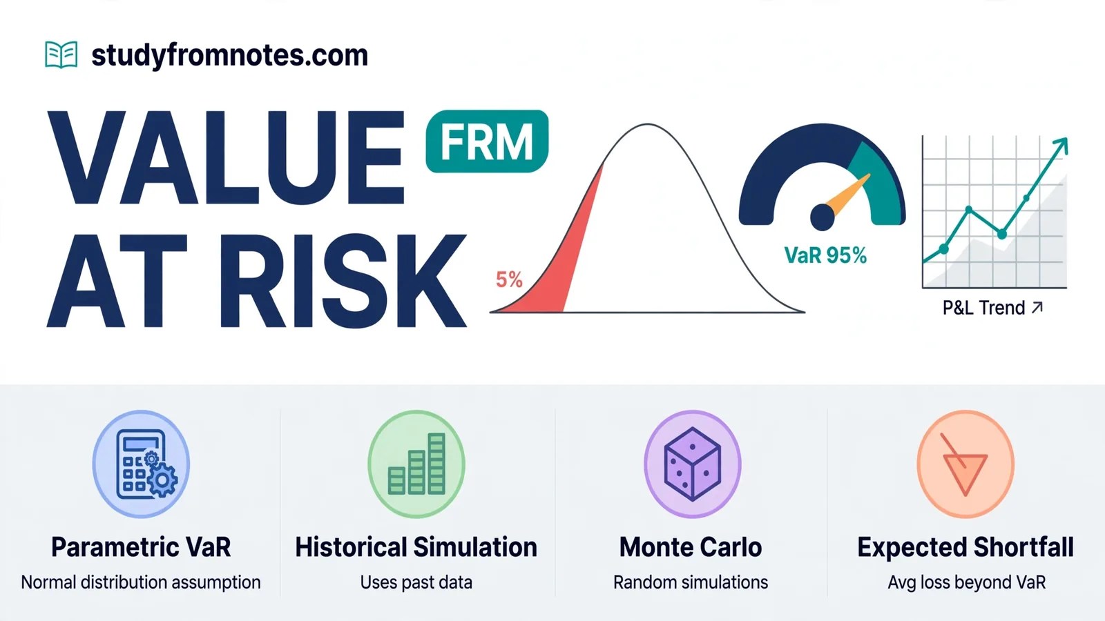
Value at Risk shows up in nearly every FRM market-risk reading, and it is one of those topics that looks simple until the exam asks you to compare three estimation methods side by side. This note covers FRM value at risk the way examiners test it: a clean definition, a worked numeric example, the three VaR methods with their trade-offs, why expected shortfall exists, how backtesting works, and the traps that catch unprepared candidates. Read it once to learn, skim the revision box before the exam.
FRM value at risk: the definition examiners expect
Value at Risk answers one question: what is the maximum loss we expect over a target time horizon, at a given confidence level? A 1-day 95% VaR of $200,000 means you are 95% confident that the portfolio will not lose more than $200,000 over the next trading day. Flip it around and the meaning gets sharper: on roughly 1 day out of 20, you expect the loss to exceed $200,000.
Three parts of that definition matter for the exam.
First, VaR is a quantile of the loss distribution, not a worst-case loss. It tells you the loss level that you cross only (1 minus confidence) of the time. Losses beyond VaR can be much larger, and VaR itself says nothing about how large they get. This single point causes more exam mistakes than anything else in the topic.
Second, you must state both the horizon and the confidence level. A “VaR of $200,000” with no horizon or confidence level is meaningless. GARP questions often test whether you notice which confidence level a number refers to before you compare two VaRs.
Third, market convention usually quotes VaR as a positive loss number. A “VaR of $197,400” means a loss of $197,400, even though the underlying return quantile is negative. Watch the sign convention in questions: a portfolio return of -1.97% at the 5th percentile is the same statement as a VaR of 1.97% of portfolio value.
FRM value at risk: a worked example (1-day, 95% parametric VaR)
Here is the classic calculation you should be able to do in under a minute.
Suppose you hold a $10 million equity portfolio. Its daily return volatility (standard deviation) is 1.2%, and you assume daily returns are normally distributed with zero mean. What is the 1-day 95% VaR?
Under the parametric approach, VaR equals the z-score for the confidence level, multiplied by the portfolio volatility, multiplied by the portfolio value:
VaR(95%) = 1.645 x 0.012 x $10,000,000 = $197,400
The 1.645 is the standard normal quantile that leaves 5% in the tail. So you can say: “We are 95% confident the portfolio will not lose more than $197,400 over the next day.” Equivalently, you expect losses to exceed $197,400 on about 5% of trading days, roughly once a month.
Two useful extensions appear constantly in questions.
Scaling across horizons: if daily returns are independent and identically distributed, VaR scales with the square root of time. A 10-day VaR equals the 1-day VaR times the square root of 10. So our $197,400 becomes about $624,200 over ten days. The square-root rule needs the iid assumption; autocorrelated returns break it.
Changing the confidence level: for 99% VaR, replace 1.645 with 2.33. The 1-day 99% VaR on this portfolio is 2.33 x 0.012 x $10,000,000 = $279,600. Examiners love asking which inputs change and which stay fixed when only the confidence level moves.
FRM value at risk: the three VaR estimation methods
Every FRM candidate must know all three methods, because comparison questions are almost guaranteed. Each method answers the same question with different assumptions.
1. Parametric VaR (delta-normal / variance-covariance)
The parametric method assumes portfolio returns follow a known distribution, almost always the normal distribution. You estimate the mean and standard deviation of returns (and the covariance matrix across positions for a multi-asset portfolio), then read the VaR straight off the distribution with a z-score. For options portfolios, the delta-normal variant approximates the option’s P&L with its delta only, which ignores gamma and breaks down for large moves.
Strengths: fast, needs little data, easy to decompose by position, and it aggregates cleanly through the covariance matrix. Weaknesses: financial returns have fat tails and skewness that the normal distribution misses, so parametric VaR understates the chance of extreme losses. It also assumes stable correlations, which tend to spike toward 1 exactly when you need diversification most.
2. Historical simulation VaR
Historical simulation makes no distributional assumption. You take the actual past returns of the portfolio (or its risk factors) over a chosen window, apply them to today’s portfolio, sort the resulting hypothetical P&L figures from worst to best, and read off the quantile. With 500 days of history and 95% confidence, the VaR is the 25th worst loss (5% of 500).
Strengths: it captures whatever fat tails, skewness, and correlation breakdowns actually occurred in the sample period, and it handles nonlinear instruments better than delta-normal. Weaknesses: it assumes the past represents the future. A calm historical window produces a VaR that collapses right before a crisis, and a short window gives a noisy, unstable estimate. It also weights every past day equally, so a regime change takes a long time to feed through.
3. Monte Carlo VaR
Monte Carlo simulation assumes a stochastic process for the risk factors (for example, geometric Brownian motion for equities) and simulates thousands of possible future paths. You reprice the full portfolio under each path, build the simulated P&L distribution, and take the quantile. For complex derivatives books, practitioners often combine Monte Carlo with full revaluation rather than delta approximations.
Strengths: it is the most flexible method. It handles path-dependent options, non-normal distributions, and any payoff structure you can model. Weaknesses: it is computationally expensive, and it replaces data risk with model risk. If your assumed process is wrong (wrong volatility dynamics, ignored jumps), the VaR is precisely wrong. Examiners often describe Monte Carlo as the most powerful and the most dangerous method at the same time.
Method comparison at a glance
| Feature | Parametric (delta-normal) | Historical simulation | Monte Carlo |
|---|---|---|---|
| Core assumption | Returns are normally distributed | Past returns represent the future | Risk factors follow an assumed stochastic process |
| Data needed | Mean, volatility, correlations | Long history of actual returns | Model parameters and calibrated processes |
| Speed | Fastest | Moderate | Slowest |
| Handles fat tails | Poorly (assumes normality) | As well as history allows | Yes, if the model includes them |
| Handles nonlinear payoffs | Poorly (delta only) | Reasonably | Best (full revaluation possible) |
| Main weakness | Understates tail risk | Backward-looking, regime changes | Model risk and computation cost |
| Best exam keyword | z-score, covariance matrix | Sorted P&L, no distribution | Simulated paths, GBM |
FRM value at risk vs expected shortfall, and coherent risk measures
Expected shortfall (ES), also called conditional VaR or tail VaR, answers the question VaR dodges: when losses exceed VaR, how bad are they on average? Formally, ES at 95% confidence is the average loss over the worst 5% of outcomes. If your 95% VaR is $197,400, the 95% ES might be $260,000. Two portfolios can share the same VaR and have very different expected shortfalls, which is exactly why regulators care about ES.
The deeper reason ES matters is coherence. Artzner and co-authors defined four axioms a sensible risk measure should satisfy: translation invariance (adding cash reduces risk one-for-one), positive homogeneity (doubling the position doubles risk), monotonicity (a portfolio that never does worse has no more risk), and subadditivity (the risk of a combined portfolio cannot exceed the sum of stand-alone risks). A measure satisfying all four is called coherent.
VaR fails subadditivity. You can construct two portfolios whose combined VaR exceeds the sum of their individual VaRs, which means VaR can penalize diversification. Expected shortfall satisfies all four axioms, so it is coherent. This is the theoretical backbone of the whole VaR-versus-ES debate, and it is a favorite exam angle: if a question asks which measure can discourage diversification, the answer is VaR.
Regulators acted on this. Under the Fundamental Review of the Trading Book, Basel replaced 99% 10-day VaR with 97.5% expected shortfall for internal market-risk models. You can read the framework in the Basel Committee’s Minimum capital requirements for market risk. For the exam, remember the pairing: 99% VaR is the old regime, 97.5% ES is the new one.
One more practical note: VaR is easier to backtest than ES because VaR produces a clean count of exceptions, while ES is an average over the tail. That is why VaR survives in risk reporting even though ES is the better measure.
FRM value at risk: backtesting VaR with the Kupiec test
Backtesting checks whether realized losses exceeded VaR roughly as often as the model predicted. Over 250 trading days, a 99% VaR should be breached about 2 to 3 times (1% of 250). If you observe 10 breaches, something is wrong with the model.
The Kupiec proportion-of-failures (POF) test formalizes this. It compares the observed exception rate (x/T) against the expected rate p using a likelihood-ratio statistic, which follows a chi-square distribution with one degree of freedom under the null hypothesis that the model is correct. A large test statistic rejects the model. You do not need to memorize the formula’s algebra for most questions, but you must know what the test does: it checks whether the exception frequency matches the VaR confidence level.
Basel wraps backtesting in a traffic-light system applied to 99% 1-day VaR over 250 days. The green zone (up to 4 exceptions) means the model looks fine. The yellow zone (5 to 9 exceptions) triggers supervisory attention and a higher capital multiplier. The red zone (10 or more exceptions) means the model is rejected and capital charges jump. The multiplier on the VaR-based capital charge ranges from 3 to 4 depending on the zone.
Two assumptions sit underneath all of this. Backtesting treats exceptions as independent Bernoulli trials, but real exceptions cluster in crises, which is why Christoffersen’s conditional-coverage test adds an independence check on top of Kupiec’s unconditional coverage. Also, backtesting needs enough data: with only a few months of history, the test has almost no power to detect a bad model.
FRM value at risk: exam traps that cost candidates marks
Read these twice. Each one maps to a question style GARP reuses.
- VaR never describes the size of tail losses. Any statement like “the most we can lose is the VaR” is false. Expected shortfall exists precisely because of this gap.
- Parametric VaR understates risk when returns have fat tails. If a question mentions kurtosis or crisis periods, the normal assumption is the weak point.
- Square-root-of-time scaling needs iid returns. Mean reversion, autocorrelation, or changing volatility all invalidate the shortcut.
- Historical simulation is only as good as its window. A VaR estimated from a calm two-year window will miss regime risk. More data is not automatically better if it spans different regimes.
- Monte Carlo output is only as good as the assumed process. Wrong model, wrong VaR, delivered with false precision.
- VaR is not subadditive, so it can rise when you diversify. If a question shows combined VaR above the sum of parts, that is the subadditivity failure, not an arithmetic error.
- Liquidity risk sits outside standard VaR. VaR assumes you can exit at market prices over the horizon. Liquidity-adjusted VaR adds an exogenous or endogenous spread cost, and examiners test whether you know plain VaR ignores it.
- VaR is procyclical. Volatility-based VaR falls in calm markets (encouraging more risk-taking) and spikes in crises (forcing sales at the worst time).
- Model risk applies to all three methods. There is no assumption-free VaR.
- In backtesting, more exceptions than expected means the model underestimates risk. Fewer exceptions can mean the model is too conservative, which wastes capital.
One-Page Revision
FRM value at risk in 60 seconds. VaR is the maximum expected loss over a horizon at a given confidence level: a quantile, not a worst case. Parametric VaR = z x sigma x portfolio value (1.645 for 95%, 2.33 for 99%), scaled by the square root of time under iid returns. Historical simulation sorts past P&L and reads the quantile with no distributional assumption. Monte Carlo simulates risk-factor paths and reprices the portfolio; flexible but model-risky. VaR ignores tail severity and fails subadditivity, so it is not coherent. Expected shortfall (average loss beyond VaR) is coherent and is Basel’s FRTB measure at 97.5%. Backtesting counts exceptions; Kupiec’s POF test checks the exception rate, and Basel’s traffic lights run green/yellow/red over 250 days at 99%. Watch for fat tails, regime changes, liquidity, and procyclicality.
Frequently asked questions
What is FRM value at risk in one sentence?
FRM value at risk is the maximum loss a portfolio is expected to suffer over a set horizon at a stated confidence level, for example “we are 95% confident daily losses will not exceed $197,400.” It is a quantile of the loss distribution, not a worst-case bound.
How do you calculate 1-day 95% parametric VaR?
Multiply the 95% z-score (1.645) by the portfolio’s daily volatility and the portfolio value. For a $10 million portfolio with 1.2% daily volatility: 1.645 x 0.012 x $10,000,000 = $197,400.
Why do regulators prefer expected shortfall over VaR?
Expected shortfall measures the average loss beyond the VaR threshold, so it captures tail severity, and it satisfies subadditivity, making it a coherent risk measure. Basel’s FRTB replaced 99% 10-day VaR with 97.5% expected shortfall for internal models.
What does the Kupiec test check?
The Kupiec proportion-of-failures test checks whether the observed number of VaR exceptions matches the exception rate implied by the confidence level, using a likelihood-ratio statistic that follows a chi-square distribution with one degree of freedom.
What are the Basel backtesting traffic-light zones?
Over 250 days at 99% confidence: green (0-4 exceptions, model acceptable), yellow (5-9, supervisory concern and higher multiplier), red (10+, model rejected). The capital multiplier ranges from 3 to 4.
Does VaR capture liquidity risk?
No. Standard VaR assumes positions can be liquidated at market prices within the horizon. Liquidity-adjusted VaR adds a cost for wide bid-ask spreads or large positions, and this distinction is a recurring exam trap.
FRM value at risk: wrapping up
If you remember nothing else, remember this chain: VaR is a quantile with a horizon and a confidence level; the three methods differ only in their assumptions about the return distribution; VaR says nothing about losses beyond itself and can punish diversification; expected shortfall fixes both problems and is the regulatory standard; and backtesting keeps every model honest. That chain answers most FRM value at risk questions you will face.
For more notes in this series, browse the Study Notes archive.


Leave a Reply