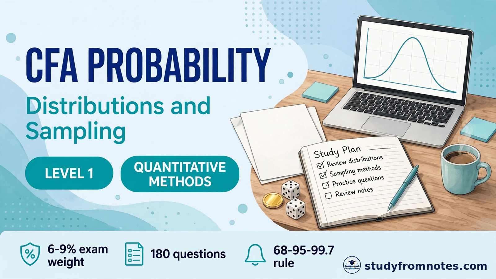
CFA Probability and Distributions Notes: Sampling, Estimation and Confidence Intervals [Level 1]

CFA probability distributions turn uncertain outcomes into numbers you can work with: the chance a trade wins, the range a return is likely to fall in, and how much you can trust a sample average. This note covers the three blocks Level 1 tests in Quantitative Methods after time value of money: probability rules, the common distributions, and sampling and estimation. Quantitative Methods carries a 6 to 9 percent weight in the 2026 CFA Level 1 exam, about 11 to 16 of the 180 questions, and rises to 11 to 14 percent from February 2027, according to CFA Institute. Start from the CFA notes hub.

CFA probability distributions: the core ideas

CFA probability distributions describe how likely each outcome is. Probability rules combine chances, the binomial and normal distributions model common outcomes, and sampling plus confidence intervals show how far a sample result can be trusted as an estimate of the whole population.

A probability is a number from 0 to 1. A random variable takes different values with different probabilities, and its probability distribution lists those values and their chances. The expected value is the probability weighted average of the outcomes, and the variance measures how spread out they are.

The November 2026 window runs 11 to 17 November, and the February 2027 window runs 22 to 28 February.

CFA probability distributions: probability rules that show up on the exam

The addition rule is P(A or B) equals P(A) plus P(B) minus P(AB). Joint probability is P(AB) equals P(A given B) times P(B). Conditional probability is P(A given B) equals P(AB) divided by P(B). If A and B are independent, P(AB) equals P(A) times P(B). Bayes formula updates a probability with new information.

Expected value is E(X) equals the sum of each outcome times its probability. Variance is the sum of each probability times the squared distance from the expected value. Covariance measures how two returns move together; correlation standardizes it to a range of minus 1 to plus 1. Chebyshev inequality works for any distribution: at least 1 minus 1 over k squared of observations lie within k standard deviations of the mean. For k equals 2, at least 75 percent lie within 2 standard deviations. It needs no normality assumption, unlike the 68-95-99.7 rule.

CFA probability distributions: the binomial distribution

The binomial distribution counts successes in a fixed number of independent trials, each with the same probability of success. It needs four conditions: fixed trials n, two outcomes per trial, constant probability of success p, and independent trials. The formula is P(X equals x) equals the combination of n choose x, times p to the power x, times (1 minus p) to the power (n minus x). The mean is np and the variance is np(1 minus p).

Worked example 1: exactly two winning trades out of five

A fund manager makes 5 independent trades, each with a 40 percent chance of profit. What is the probability that exactly 2 of the 5 trades are profitable? Here n equals 5, x equals 2, and p equals 0.40. The combination C(5,2) equals 10. Then p squared is 0.16, and (1 minus p) cubed is 0.216. Multiply: 10 times 0.16 times 0.216 equals 0.3456, or about 34.56 percent. The expected number of profitable trades is np, which is 2.0, and the variance is np(1 minus p), which is 1.2.

CFA probability distributions: normal and lognormal

The normal distribution is continuous, symmetric, and fully described by its mean and variance. About 68 percent lie within one standard deviation of the mean, about 90 percent within 1.65, about 95 percent within 1.96, and about 99 percent within 2.58. The rounded 68-95-99.7 rule is the quick version the exam expects you to recall.

The lognormal distribution cannot be negative and is positively skewed. If X is lognormal, the natural log of X is normally distributed. That makes it the right model for asset prices, which cannot fall below zero, but the wrong model for asset returns, which can be negative. The exam tests this distinction directly: prices are lognormal, returns are closer to normal.

CFA probability distributions: the t, chi-square and F distributions

The Student t-distribution has one parameter, degrees of freedom equal to n minus 1. It is bell shaped like the normal distribution but has fatter tails and a lower peak, and it approaches the normal distribution as degrees of freedom rise. Use it for a single mean when the population variance is unknown, especially with small samples below 30.

Distribution	Defined by	Use it for
Student t	Degrees of freedom, n minus 1	Single mean, variance unknown, small samples
Chi-square	Degrees of freedom, n minus 1	Test of a single variance
F	Two degrees of freedom	Test of equality of two variances

The chi-square distribution is the sum of squares of independent standard normal variables, so it cannot be negative. The F-distribution is the ratio of two chi-square distributions, so it also cannot be negative; use it with F equal to the larger sample variance divided by the smaller one.

CFA probability distributions: sampling and the central limit theorem

A population is every item of interest; a sample is the part you actually observe. Sampling error is the sample mean minus the population mean: the gap between what you measured and the truth. The standard error of the mean measures how far sample means typically fall from the population mean. If the population variance is known, the standard error is sigma divided by the square root of n. If it is unknown, use the sample standard deviation s divided by the square root of n. Quadrupling the sample size only halves the standard error.

The central limit theorem is the reason sampling works. For simple random samples, the sampling distribution of the sample mean approaches a normal distribution with mean mu and variance sigma squared over n as n grows. A sample of 30 or more is typically treated as large enough.

Simple random sampling gives every item an equal chance of inclusion. Stratified random sampling divides the population into subgroups, or strata, then draws a random sample from each; it cuts sampling error when strata are homogeneous inside and different from each other. Convenience and judgmental sampling are non-probability methods and carry selection bias risk.

CFA probability distributions: confidence intervals

A confidence interval has the form point estimate plus or minus the reliability factor times the standard error. The reliability factors are 1.645 for 90 percent confidence, 1.96 for 95 percent, and 2.575 for 99 percent. When the population variance is known, use z for any sample size. When it is unknown and n is below 30, use t with n minus 1 degrees of freedom. A 95 percent interval means 95 percent of intervals built this way contain the true mean, not a 95 percent chance for this one interval.

Worked example 2: a 95 percent confidence interval for a fund return

A sample of 36 monthly fund returns has a mean of 12 percent and a standard deviation of 6 percent. Build the 95 percent confidence interval for the population mean return. The standard error is s divided by the square root of n, which is 6 divided by the square root of 36, or 6 divided by 6, which is 1.0. The reliability factor for 95 percent confidence is z equals 1.96, so the margin of error is 1.96 times 1.0, or 1.96. The interval is 12 plus or minus 1.96, which is (10.04 percent, 13.96 percent).

Two exam follow-ups. First, with the t-distribution (35 degrees of freedom, t equals 2.0301) the interval would be slightly wider, (9.97 percent, 14.03 percent), because the t-distribution has fatter tails.

CFA probability distributions: exam traps

Trap 1: using the normal rule on a non-normal distribution. The 68-95-99.7 rule needs normality; otherwise use Chebyshev.

Trap 2: lognormal for returns. Asset prices are lognormal; returns can be negative, so they are not. The exam asks this both ways.

Trap 3: z when the question needs t. Variance unknown and n below 30 means t, not z.

Trap 4: confusing sampling error with standard error. Sampling error is one sample mean minus the population mean.

Trap 5: reading a confidence interval as a probability. A 95 percent interval describes the method, not this one interval.

Trap 6: forgetting the square root in the standard error. Standard error falls with the square root of n, not with n.

Trap 7: dependent trials in the binomial. The binomial needs independent trials with constant p.

CFA probability distributions: one-page revision box

Formula or rule	What it is
P(A or B) = P(A) + P(B) – P(AB)	Addition rule
P(X = x) = C(n,x) p^x (1 – p)^(n – x)	Binomial probability
68% / 95% / 99.7% within 1 / 2 / 3 sd	Normal 68-95-99.7 rule
SE = s / sqrt(n)	Standard error of the mean
CI = x-bar +/- z x SE (known variance)	Confidence interval, z
CI = x-bar +/- t x SE, df = n – 1	Confidence interval, t

The companion note is at CFA Quantitative Methods: time value of money and hypothesis testing. For the full Level 1 set, return to the CFA notes hub.

Sources

CFA Institute, CFA Program Level I exam page (exam structure, 2026 and 2027 topic weights). 300hours, CFA Level 1 Quantitative Methods cheat sheet. AnalystNotes, binomial distribution and confidence interval notes. 365 Financial Analyst, Quantitative Methods formulas. Kaplan Schweser Reading 7 notes via EduRev. Analyst Dojo, Quintedge and Soleadea (2026 and 2027 exam windows and fees).